Listings, figures and delivery
A listing shows records, not statistics: every serious adverse event, every death, every protocol deviation. A reviewer reads it line by line. A figure shows a pattern that a table hides: a trend over the visits, or how fast events happen. This chapter makes one listing and two figures. Then it delivers a data set in the format that a regulator reads: the SAS transport file, XPT.
As in chapter 13, the programs read pharmaverseadam and save their files to programs/output/.
14.1 A listing by hand
Section titled “14.1 A listing by hand”# Chapter 14: a listing of serious adverse events, printed and written to Wordlibrary(dplyr)library(flextable)library(officer)
cols <- c( "Placebo" = "Placebo", "Xanomeline Low Dose" = "Xanomeline Low Dose", "Xanomeline High Dose" = "Xanomeline High Dose")sae <- pharmaverseadam::adae |> filter(SAFFL == "Y", AESER == "Y") |> mutate(TRT = factor(TRT01A, levels = cols)) |> arrange(TRT, USUBJID, ASTDT, AEDECOD) |> select(TRT, USUBJID, AEDECOD, ASTDT, AENDT, AESEV, AEOUT)
nrow(sae)#> [1] 3options(width = 110) # a listing is wide: landscape in Wordsae |> select(TRT, USUBJID, AEDECOD, ASTDT, AESEV) |> as.data.frame() |> print(right = FALSE, row.names = FALSE)#> TRT USUBJID AEDECOD ASTDT AESEV#> Xanomeline Low Dose 01-709-1424 SYNCOPE 2013-03-07 MODERATE#> Xanomeline Low Dose 01-718-1170 SYNCOPE 2013-10-12 SEVERE#> Xanomeline High Dose 01-718-1371 PARTIAL SEIZURES WITH SECONDARY GENERALISATION 2013-06-02 SEVERE
# the listing: a value of TRT and USUBJID once per group, wrapped textft <- sae |> mutate(TRT = as.character(TRT)) |> flextable() |> set_header_labels( TRT = "Treatment", USUBJID = "Subject", AEDECOD = "Preferred term", ASTDT = "Start", AENDT = "End", AESEV = "Severity", AEOUT = "Outcome" ) |> merge_v(j = c("TRT", "USUBJID")) |> valign(valign = "top", part = "body") |> width(j = c("TRT", "AEDECOD", "AEOUT"), width = c(1.6, 2.4, 1.8)) |> add_footer_lines(paste("Records listed:", nrow(sae))) |> theme_booktabs()
landscape <- prop_section(page_size = page_size(orient = "landscape"))save_as_docx( "Listing 16.2.7 Serious adverse events (safety population)" = ft, path = "output/l_16_2_7_sae.docx", pr_section = landscape)file.exists("output/l_16_2_7_sae.docx")#> [1] TRUEThe safety population has 3 serious adverse events, and the listing shows all 3. Nobody on placebo had one. Subject 01-709-1424 was randomised to the high dose but is listed under the low dose: a safety listing shows the actual treatment (chapter 13).
A listing has two parts. The records come from dplyr, and the page comes from flextable:
arrange()decides the order of the lines: treatment, subject, start date. The factorTRTputs the treatments in the order of the study, not in alphabetical order.print()in the console is for you.options(width = 110)keeps each record on one line of the screen.flextable()makes the table for Word.set_header_labels()gives the columns their titles.merge_v()merges the cells ofTRTandUSUBJIDwith the same value, so a treatment prints once for its subjects.valign(valign = "top")puts the merged text at the top.width()gives the long columns more room. A long preferred term wraps inside its cell; the line never runs off the page.add_footer_lines()writes how many records the listing has. A reader can check it against the data.save_as_docx()writes the Word file.prop_section()from officer makes the page landscape, and the name of the argument becomes the title above the table.
Exercise 14-1. List the deaths of the safety population (DTHFL == "Y" in ADSL) with treatment, age, sex, the date of the last dose (TRTEDT), the date of death and its cause. How many deaths are there per treatment?
14.2 The numbers of a figure
Section titled “14.2 The numbers of a figure”A figure is a picture of numbers. Compute the numbers first, check them, and only then draw them. The first figure shows the mean change from baseline in weight at each visit, with the standard error (SE) of the mean: the standard deviation divided by the square root of n. It shows how precise the mean is.
# Chapter 14: the numbers of a figure: mean change in weight per visitlibrary(dplyr)
weight <- pharmaverseadam::advs |>  filter(SAFFL == "Y", PARAMCD == "WEIGHT", ANL01FL == "Y", AVISITN %in% 2:26)
# one record per subject and visit? not here: check before you take a meanweight |>  count(USUBJID, AVISITN) |>  count(records = n)#> # A tibble: 1 x 2#>   records     n#>     <int> <int>#> 1       2  1409weight |>  filter(USUBJID == "01-701-1015", AVISITN == 2) |>  select(USUBJID, AVISIT, AVAL, CHG, DTYPE)#> # A tibble: 2 x 5#>   USUBJID     AVISIT  AVAL   CHG DTYPE#>   <chr>       <chr>  <dbl> <dbl> <chr>#> 1 01-701-1015 Week 2  53.1 -1.36 <NA>#> 2 01-701-1015 Week 2  53.1 -1.36 AVERAGE
# DTYPE = "AVERAGE" is a derived copy of the same value: keep the collected onemeans <- weight |>  filter(is.na(DTYPE)) |>  group_by(TRTA, AVISITN) |>  summarise(    n = n(), mean = mean(CHG), se = sd(CHG) / sqrt(n()),    .groups = "drop"  )saveRDS(means, "output/vs_means.rds")
means |>  filter(AVISITN == 24) |>  mutate(across(c(mean, se), \(x) round(x, 2)))#> # A tibble: 3 x 5#>   TRTA                 AVISITN     n  mean    se#>   <chr>                  <dbl> <int> <dbl> <dbl>#> 1 Placebo                   24    59  0.15  0.3#> 2 Xanomeline High Dose      24    28  0.92  1.26#> 3 Xanomeline Low Dose       24    25 -0.43  0.42
Check the records first. count(USUBJID, AVISITN) counts the records per subject and visit, and the second count() counts those counts. Every one of the 1409 subject-visits has 2 records. Subject 01-701-1015 shows why: at week 2 there is the collected weight, and a second record with DTYPE = "AVERAGE", a derived record with the same value. With both records, every subject counts twice in n, and the standard error is too small. filter(is.na(DTYPE)) keeps the collected record.
summarise() then gives n, the mean and the SE per treatment and visit. At week 24, placebo has 59 subjects with a mean change of 0.15 kg (SE 0.3). The low dose has only 25 subjects and the high dose 28: many subjects of the active arms stopped early. A mean of few subjects needs this warning next to it.
14.3 A line plot with ggplot2
Section titled “14.3 A line plot with ggplot2”# Chapter 14: a line plot of mean change from baseline, with error barslibrary(dplyr)library(ggplot2)
means <- readRDS("output/vs_means.rds") |> # made by 14_2 mutate(TRTA = factor( TRTA, c("Placebo", "Xanomeline Low Dose", "Xanomeline High Dose") ))
fig <- ggplot(means, aes(x = AVISITN, y = mean, colour = TRTA)) + geom_hline(yintercept = 0, colour = "grey60") + geom_line(position = position_dodge(width = 0.6)) + geom_point(position = position_dodge(width = 0.6)) + geom_errorbar( aes(ymin = mean - se, ymax = mean + se), width = 0.8, position = position_dodge(width = 0.6) ) + scale_x_continuous(breaks = c(2, 4, 6, 8, 12, 16, 20, 24, 26)) + labs( title = "Mean change from baseline in weight (kg), mean and standard error", x = "Week", y = "Change from baseline (kg)", colour = NULL ) + theme_bw() + theme(legend.position = "bottom")fig#> [figure 1: /figs/14_3_vs_plot-1.png]
# the file for the report: 8 by 5 inches, 300 dots per inchggsave("output/f_14_2_1_weight.png", fig, width = 8, height = 5, dpi = 300)file.exists("output/f_14_2_1_weight.png")#> [1] TRUE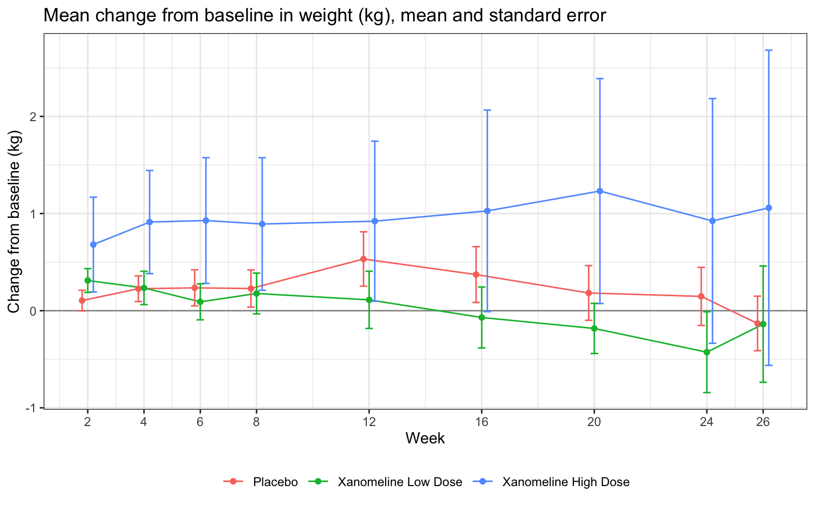
ggplot2 builds a plot in layers, joined with +:
-
ggplot(means, aes(...))names the data and the aesthetics: which column goes on the x axis, which on the y axis, and which column gives the colour. -
Each
geom_function adds a layer:geom_hline()the line at 0,geom_line()the lines,geom_point()the points,geom_errorbar()the bars from mean − SE to mean + SE. -
position_dodge(width = 0.6)moves the three treatments a little to the side, so the bars do not hide each other. Every layer uses the same dodge, so each bar stays on its point. -
scale_x_continuous(breaks = ...)puts a tick at each planned week.labs()sets the title and the axis titles.theme_bw()andtheme()set the look. -
fig <- ggplot(...)keeps the plot in a variable.figon its own line draws it.ggsave()writes it to a file: here a PNG image of 8 by 5 inches with 300 dots per inch, the size for a report page. The file type comes from the file name:.pdfor.svgwork too.
Check the plot against the table of 14.2: at week 24 the placebo point is at 0.15. The long bars of the high dose show how few subjects are left.
Exercise 14-2. Make the same figure for systolic blood pressure after lying down for 5 minutes (PARAMCD == "SYSBP", ATPT == "AFTER LYING DOWN FOR 5 MINUTES"). What are n and the mean change at week 24 per treatment?
14.4 Time to event: the data
Section titled “14.4 Time to event: the data”The second figure is a Kaplan-Meier plot of the time to the first dermatologic event: an application site reaction or a skin event. Xanomeline is given as a skin patch, so these events matter for its safety. It needs an ADTTE data set. pharmaverseadam has adtte_onco for the pilot subjects, but its parameters are made-up oncology endpoints (overall survival, progression-free survival). Chapter 12 builds the real ADTTE. So that this chapter runs on its own, the program derives the parameter in a few lines.
Three words first. The event is what you wait for: here the first dermatologic TEAE. A subject without the event is censored: you know only that the event did not happen before a date, here the end of the study. CNSR is 0 for an event and 1 for a censored subject. AVAL is the time in days from the first dose.
# Chapter 14: time to the first dermatologic event, and its medianlibrary(dplyr)library(survival)
adsl <- pharmaverseadam::adsl |>  filter(SAFFL == "Y") |>  mutate(TRT = factor(    TRT01A, c("Placebo", "Xanomeline Low Dose", "Xanomeline High Dose")  ))
# the event: the first treatment-emergent AE of the dermatologic queryfirst_derm <- pharmaverseadam::adae |>  filter(    TRTEMFL == "Y",    grepl("APPLICATION|DERMATITIS|ERYTHEMA|BLISTER", AEDECOD) |      (AEBODSYS == "SKIN AND SUBCUTANEOUS TISSUE DISORDERS" &        !AEDECOD %in% c("COLD SWEAT", "HYPERHIDROSIS", "ALOPECIA"))  ) |>  group_by(USUBJID) |>  summarise(EVNTDT = min(ASTDT))
# no event: censored at the end of study. AVAL in days from the first dosettde <- adsl |>  left_join(first_derm, by = "USUBJID") |>  mutate(    CNSR = if_else(is.na(EVNTDT), 1, 0),    ADT = coalesce(EVNTDT, EOSDT),    AVAL = as.numeric(ADT - TRTSDT) + 1  ) |>  select(USUBJID, TRT, TRTSDT, ADT, AVAL, CNSR)saveRDS(ttde, "output/ttde.rds")
ttde |> filter(USUBJID == "01-701-1015")#> # A tibble: 1 x 6#>   USUBJID     TRT     TRTSDT     ADT         AVAL  CNSR#>   <chr>       <fct>   <date>     <date>     <dbl> <dbl>#> 1 01-701-1015 Placebo 2014-01-02 2014-01-03     2     0ttde |> count(TRT, event = CNSR == 0)#> # A tibble: 6 x 3#>   TRT                  event     n#>   <fct>                <lgl> <int>#> 1 Placebo              FALSE    57#> 2 Placebo              TRUE     29#> 3 Xanomeline Low Dose  FALSE    33#> 4 Xanomeline Low Dose  TRUE     63#> 5 Xanomeline High Dose FALSE    13#> 6 Xanomeline High Dose TRUE     59
# Kaplan-Meier: Surv() wants the event as 1, so give it 1 - CNSRkm <- survfit(Surv(AVAL, 1 - CNSR) ~ TRT, data = ttde)km#> Call: survfit(formula = Surv(AVAL, 1 - CNSR) ~ TRT, data = ttde)#>#> n events median 0.95LCL 0.95UCL#> TRT=Placebo 86 29 NA NA NA#> TRT=Xanomeline Low Dose 96 63 34 28 51#> TRT=Xanomeline High Dose 72 59 31 23 46first_dermkeeps the TEAEs of the pilot study’s dermatologic query: the preferred terms with APPLICATION, DERMATITIS, ERYTHEMA or BLISTER, and the skin SOC without three terms.min(ASTDT)takes the first event of each subject.left_join()keeps every subject of ADSL. A subject without an event getsNA, thenCNSR = 1and the end of study date.AVALcounts the day of the first dose as day 1. Subject 01-701-1015 had an event on the second day:AVAL = 2,CNSR = 0.
29 of the 86 subjects on placebo had the event, 63 of 96 on the low dose and 59 of 72 on the high dose.
survfit() from the survival package estimates the Kaplan-Meier curve: for each day, the fraction of subjects still without the event. Surv(AVAL, 1 - CNSR) describes the time and the event; Surv() wants 1 for an event, so it gets 1 - CNSR. The median time to the event is 34 days on the low dose (95% confidence interval 28 to 51) and 31 days on the high dose (23 to 46). On placebo it is NA: fewer than half of the subjects had the event, so the curve never falls to 50%. A table must say “not reached”, not “NA”.
14.5 A Kaplan-Meier plot
Section titled “14.5 A Kaplan-Meier plot”# Chapter 14: a Kaplan-Meier plot with the number of subjects at risklibrary(dplyr)library(ggsurvfit)
ttde <- readRDS("output/ttde.rds") # made by 14_4
km <- survfit2(Surv(AVAL, 1 - CNSR) ~ TRT, data = ttde)
# the numbers under the plot: subjects at risk at day 0, 30, 60, ...tidy_survfit(km, times = seq(0, 180, by = 30)) |> select(strata, time, n.risk) |> tidyr::pivot_wider(names_from = strata, values_from = n.risk)#> # A tibble: 7 x 4#> time Placebo `Xanomeline High Dose` `Xanomeline Low Dose`#> <dbl> <dbl> <dbl> <dbl>#> 1 0 86 72 96#> 2 30 69 38 42#> 3 60 59 15 20#> 4 90 49 7 13#> 5 120 45 5 8#> 6 150 40 5 6#> 7 180 35 3 5
ggsurvfit(km) + add_censor_mark() + add_risktable(times = seq(0, 180, by = 30), risktable_stats = "n.risk") + scale_x_continuous(breaks = seq(0, 180, by = 30)) + labs( title = "Time to first dermatologic event (safety population)", x = "Days since first dose", y = "Probability without event" ) + theme(legend.position = "bottom")#> [figure 1: /figs/14_5_km-1.png]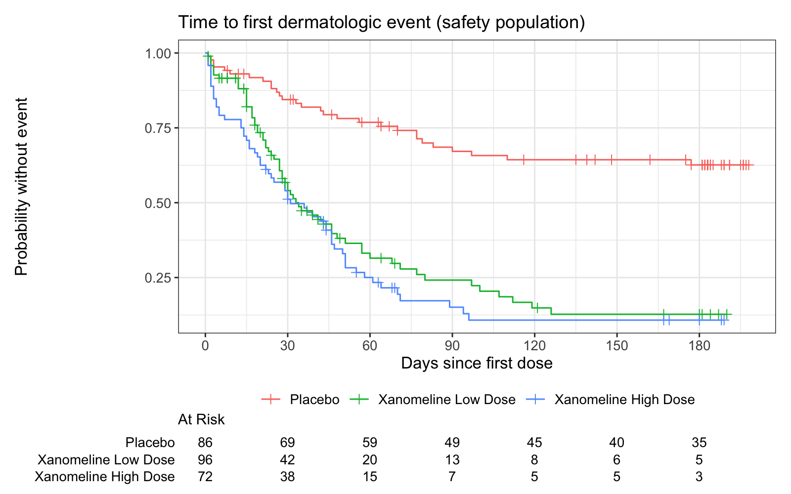
survfit2()from ggsurvfit issurvfit()that keeps the names of the data, so the legend saysPlacebo, notTRT=Placebo.ggsurvfit()draws the curves,add_censor_mark()a+for each censored subject, andadd_risktable()the number of subjects at risk under the plot: the subjects without the event and not yet censored on that day.tidy_survfit()gives the same numbers as a data frame, so you can check them. At day 90, 49 subjects on placebo are still at risk; on the low dose 13 and on the high dose 7.
It is a ggplot, so scale_x_continuous(), labs() and theme() work as in 14.3.
Exercise 14-3. The risk table says 49 placebo subjects are at risk at day 90. Check it with dplyr on the data of 14.4.
14.6 Delivery: a data set as an XPT file
Section titled “14.6 Delivery: a data set as an XPT file”A study sends its SDTM and ADaM data sets to the regulator as SAS transport files, version 5: XPT. Each variable has a name, a type, a length and a label, and each value must fit its length. These attributes come from the ADaM specification, one row per variable. xportr applies a specification to a data frame and writes the file.
# Chapter 14: write a SAS transport file (XPT) with xportr, read it backlibrary(dplyr)library(xportr)
# the specification: one row per variable, as in the ADaM specificationspec <- tribble(  ~dataset, ~variable, ~order, ~type, ~length, ~format, ~label,  "ADSL", "STUDYID", 1, "character", 12, NA, "Study Identifier",  "ADSL", "USUBJID", 2, "character", 11, NA, "Unique Subject Identifier",  "ADSL", "TRT01A", 3, "character", 20, NA, "Actual Treatment for Period 01",  "ADSL", "AGE", 4, "integer", 8, NA, "Age",  "ADSL", "SEX", 5, "character", 1, NA, "Sex",  "ADSL", "TRTSDT", 6, "integer", 8, "DATE9.", "Date of First Exposure",  "ADSL", "SAFFL", 7, "character", 1, NA, "Safety Population Flag")
adsl <- pharmaverseadam::adsl |>  filter(SAFFL == "Y") |>  select(USUBJID, STUDYID, AGE, SEX, TRT01A, TRTSDT, SAFFL)
adsl |>  xportr_metadata(spec, domain = "ADSL") |>  xportr_type() |>  xportr_length() |>  xportr_label() |>  xportr_format() |>  xportr_order() |>  xportr_df_label(    tibble(dataset = "ADSL", label = "Subject-Level Analysis Dataset")  ) |>  xportr_write("output/adsl.xpt")#>#> -- All variables in dataset are found in `metadata` --#>#> -- 5 reordered in dataset --#>
# read the file back: the values (haven), then what the file says (foreign)haven::read_xpt("output/adsl.xpt") |>  filter(USUBJID == "01-701-1015")#> # A tibble: 1 x 7#>   STUDYID      USUBJID     TRT01A    AGE SEX   TRTSDT     SAFFL#>   <chr>        <chr>       <chr>   <dbl> <chr> <date>     <chr>#> 1 CDISCPILOT01 01-701-1015 Placebo    63 F     2014-01-02 Y
file <- foreign::lookup.xport("output/adsl.xpt")$adsltibble( name = file$name, type = file$type, length = file$width, format = file$format, label = file$label)#> # A tibble: 7 x 5#> name type length format label#> <chr> <chr> <int> <chr> <chr>#> 1 STUDYID character 12 "" Study Identifier#> 2 USUBJID character 11 "" Unique Subject Identifier#> 3 TRT01A character 20 "" Actual Treatment for Period 01#> 4 AGE numeric 8 "" Age#> 5 SEX character 1 "" Sex#> 6 TRTSDT numeric 8 "DATE" Date of First Exposure#> 7 SAFFL character 1 "" Safety Population Flagspecis a small specification, written in the program withtribble()(a tibble written row by row). At work you read it from the specification file, for example withreadxl.xportr_metadata()attaches the specification and the data set name, so the next functions need no arguments.xportr_type()converts each column to the type of the specification.xportr_length()sets the lengths,xportr_label()the labels andxportr_format()the SAS formats, such asDATE9.for a date.xportr_order()puts the columns in the order of the specification. The message5 reordered in datasettells you that it moved them: the data hadUSUBJIDfirst.xportr_df_label()gives the data set its label, andxportr_write()writesoutput/adsl.xpt.
Read the file back. haven::read_xpt() reads the values: subject 01-701-1015, 63 years old, TRTSDT still a date. foreign::lookup.xport() shows what the file says about each column: TRT01A is character with length 20, TRTSDT is numeric with the format DATE, and each column has its label. These are the attributes that define.xml describes.
Exercise 14-4. Give TRT01A the length 10 in the specification and write the file again. What does R say, and what length does the file have?
14.7 Before you send a file
Section titled “14.7 Before you send a file”Each output of this part is now a file in programs/output/:
| Output | Package | Function | File |
|---|---|---|---|
| Table | gt, flextable, officer | gtsave(), body_add_flextable() |
t_14_1_1_demog.html, .docx |
| Listing | flextable, officer | save_as_docx() |
l_16_2_7_sae.docx |
| Figure | ggplot2 | ggsave() |
f_14_2_1_weight.png |
| Data set | xportr | xportr_write() |
adsl.xpt |
Before a file leaves your hands, open it and check four things:
- The numbers. The big N in the header matches ADSL. The count in the footer of a listing matches the data.
- The page. No column is cut, and a long text wraps inside its cell.
- The title. It has the number and the population of the shell.
- The source. A program made the file, and the program is the version in your study folder. Never edit an output by hand: the next run overwrites your change, and nobody can reproduce it.
14.8 Summary
Section titled “14.8 Summary”- A listing shows records. Sort them with
arrange(), then make the page with flextable:merge_v()prints a value once per group,save_as_docx()writes Word. - Compute the numbers of a figure first, and print them. Count the records per subject and visit before a mean.
- ggplot2 builds a plot in layers: data and aesthetics, then
geom_layers, scales, labels and a theme. Surv(AVAL, 1 - CNSR): R wants the event as 1.survfit()gives the Kaplan-Meier estimate and the median; a median that isNAis “not reached”.- ggsurvfit draws the Kaplan-Meier plot with the subjects at risk.
tidy_survfit()gives the same numbers to check. - xportr applies a specification (type, length, label, format, order) and writes an XPT file. Read it back with haven.
- Write every output with a program, then open the file and check it.
14.9 Exercises
Section titled “14.9 Exercises”Exercises 14-1 to 14-4 are in the sections above:
- Exercise 14-1 (14.1): a listing of the deaths.
- Exercise 14-2 (14.3): the figure for systolic blood pressure.
- Exercise 14-3 (14.5): the subjects at risk at day 90, from the data.
- Exercise 14-4 (14.6): a length that is too short.
The answers are in Answers, Part III.
Found an error or have a question? Write to datastep.studio@gmail.com· Every program runs in DataStep Studio for R, the R extension for VS Code and Positron.
Data: the CDISC pilot study (cdiscpilot01), from the R packagespharmaversesdtm andpharmaverseadam (Apache License 2.0).
R is a project of the R Foundation. SAS and all other SAS Institute Inc. product or service names are registered trademarks or trademarks of SAS Institute Inc. This book is not affiliated with or endorsed by SAS Institute Inc. or the R Foundation. CDISC, SDTM and ADaM are trademarks of the Clinical Data Interchange Standards Consortium.
© 2026 DataStep Labs. All rights reserved.