Answers, Part III (chapters 13 and 14)
Each answer has a program that was run, and its output. Try the exercise yourself first. Then compare your numbers with the numbers here. A different program that gives the same numbers is also a right answer.
Chapter 13
Section titled “Chapter 13”Exercise 13-1
Section titled “Exercise 13-1”# Answer 13-1: the ethnicity section of the demographics tablelibrary(dplyr)library(tidyr)
round_half_up <- function(x, digits = 0) { scale <- 10^digits sign(x) * floor(abs(x) * scale + 0.5 + 1e-9) / scale}n_pct <- function(n, N) sprintf("%d (%.1f%%)", n, round_half_up(100 * n / N, 1))
cols <- c( "Placebo" = "Placebo", "Low Dose" = "Xanomeline Low Dose", "High Dose" = "Xanomeline High Dose", "Total" = "Total")saf <- pharmaverseadam::adsl |> filter(SAFFL == "Y")adsl <- bind_rows(saf, mutate(saf, TRT01A = "Total")) |> mutate(TRT = factor(TRT01A, levels = cols, labels = names(cols)))bign <- count(adsl, TRT, name = "N")
adsl |> count(TRT, label = ETHNIC) |> complete(TRT, label, fill = list(n = 0)) |> left_join(bign, by = "TRT") |> mutate(value = n_pct(n, N)) |> select(label, TRT, value) |> pivot_wider(names_from = TRT, values_from = value)#> # A tibble: 2 x 5#> label Placebo `Low Dose` `High Dose` Total#> <chr> <chr> <chr> <chr> <chr>#> 1 HISPANIC OR LATINO 3 (3.5%) 6 (6.3%) 3 (4.2%) 12 (4.7%)#> 2 NOT HISPANIC OR LATINO 83 (96.5%) 90 (93.8%) 69 (95.8%) 242 (95.3%)12 subjects are Hispanic or Latino: 3 on placebo, 6 on the low dose and 3 on the high dose. The section is the same code as age group, sex and race in 13.2: count, complete(), join the big N, format. In 13_2_demog_hand.R you add one line, Ethnicity = factor(ETHNIC), to the transmute(), and the name to the order of the sections.
Exercise 13-2
Section titled “Exercise 13-2”# Answer 13-2: subjects with at least one serious TEAE, with the zeroslibrary(dplyr)library(tidyr)
cols <- c( "Placebo" = "Placebo", "Low Dose" = "Xanomeline Low Dose", "High Dose" = "Xanomeline High Dose")bign <- pharmaverseadam::adsl |> filter(SAFFL == "Y") |> mutate(TRT = factor(TRT01A, levels = cols, labels = names(cols))) |> count(TRT, name = "N")
pharmaverseadam::adae |> filter(SAFFL == "Y", TRTEMFL == "Y", AESER == "Y") |> mutate(TRT = factor(TRT01A, levels = cols, labels = names(cols))) |> distinct(TRT, USUBJID) |> count(TRT) |> complete(TRT, fill = list(n = 0)) |> left_join(bign, by = "TRT") |> mutate(pct = round(100 * n / N, 1))#> # A tibble: 3 x 4#> TRT n N pct#> <fct> <int> <int> <dbl>#> 1 Placebo 0 86 0#> 2 Low Dose 2 96 2.1#> 3 High Dose 1 72 1.42 subjects on the low dose and 1 on the high dose had at least one serious TEAE. Nobody on placebo had one. Without complete(), the placebo line would not exist at all, and a table would show a blank instead of 0. complete(TRT) works here because TRT is a factor: it knows all three levels, also the one with no row.
Exercise 13-3
Section titled “Exercise 13-3”# Answer 13-3: the three system organ classes with the most subjectslibrary(dplyr)
pharmaverseadam::adae |> filter(SAFFL == "Y", TRTEMFL == "Y") |> distinct(AEBODSYS, USUBJID) |> count(AEBODSYS, sort = TRUE) |> head(3)#> # A tibble: 3 x 2#> AEBODSYS n#> <chr> <int>#> 1 GENERAL DISORDERS AND ADMINISTRATION SITE CONDITIONS 108#> 2 SKIN AND SUBCUTANEOUS TISSUE DISORDERS 98#> 3 NERVOUS SYSTEM DISORDERS 53GENERAL DISORDERS AND ADMINISTRATION SITE CONDITIONS (108 subjects), SKIN AND SUBCUTANEOUS TISSUE DISORDERS (98) and NERVOUS SYSTEM DISORDERS (53). distinct(AEBODSYS, USUBJID) keeps one row per subject and SOC, so count() counts subjects. sort = TRUE sorts the result, the most frequent first. 108 is also the Total of the second line of the table in 13.4.
Exercise 13-4
Section titled “Exercise 13-4”# Answer 13-4: the percents where round() and round_half_up() differlibrary(dplyr)library(tidyr)options(width = 90) # the table is wider than 80 characters
round_half_up <- function(x, digits = 0) { scale <- 10^digits sign(x) * floor(abs(x) * scale + 0.5 + 1e-9) / scale}
saf <- pharmaverseadam::adsl |> filter(SAFFL == "Y")adsl <- bind_rows(saf, mutate(saf, TRT01A = "Total"))
adsl |> select(TRT01A, AGEGR1, SEX, RACE) |> pivot_longer(-TRT01A, names_to = "variable", values_to = "value") |> count(TRT01A, variable, value) |> group_by(TRT01A, variable) |> mutate(N = sum(n)) |> ungroup() |> mutate( pct = 100 * n / N, r = sprintf("%.1f", round(pct, 1)), half_up = sprintf("%.1f", round_half_up(pct, 1)) ) |> filter(r != half_up)#> # A tibble: 1 x 8#> TRT01A variable value n N pct r half_up#> <chr> <chr> <chr> <int> <int> <dbl> <chr> <chr>#> 1 Xanomeline Low Dose RACE BLACK OR AFRICAN AMERICAN 6 96 6.25 6.2 6.3Only one percent differs: the 6 Black or African American subjects of the 96 on the low dose. The percent is exactly 6.25. round() gives 6.2, round_half_up() gives 6.3. Every other percent is not exactly halfway, so both rules give the same text. One cell in 44 is enough to make a comparison of two tables fail.
Exercise 13-5
Section titled “Exercise 13-5”# Answer 13-5: the TEAE table for severe events only, with tbl_hierarchical()library(dplyr)library(gtsummary)
cols <- c( "Placebo" = "Placebo", "Low Dose" = "Xanomeline Low Dose", "High Dose" = "Xanomeline High Dose")adsl <- pharmaverseadam::adsl |> filter(SAFFL == "Y") |> mutate(TRT = factor(TRT01A, levels = cols, labels = names(cols)))
pharmaverseadam::adae |> filter(SAFFL == "Y", TRTEMFL == "Y", AESEV == "SEVERE") |> mutate(TRT = factor(TRT01A, levels = cols, labels = names(cols))) |> tbl_hierarchical( variables = c(AEBODSYS, AEDECOD), by = TRT, id = USUBJID, denominator = adsl, overall_row = TRUE, label = list(..ard_hierarchical_overall.. = "ANY SEVERE TEAE") ) |> sort_hierarchical() |> as_tibble(col_labels = FALSE) |> mutate(label = stringr::str_trunc(label, 40)) |> head(4)#> # A tibble: 4 x 4#> label stat_1 stat_2 stat_3#> <chr> <chr> <chr> <chr>#> 1 ANY SEVERE TEAE 5 (5.8%) 16 (17%) 8 (11%)#> 2 GENERAL DISORDERS AND ADMINISTRATION ... 0 (0%) 7 (7.3%) 0 (0%)#> 3 APPLICATION SITE IRRITATION 0 (0%) 3 (3.1%) 0 (0%)#> 4 APPLICATION SITE ERYTHEMA 0 (0%) 2 (2.1%) 0 (0%)5 subjects on placebo, 16 on the low dose and 8 on the high dose had at least one severe TEAE. These are the numbers of exercise 1-4. The program uses the default statistic of tbl_hierarchical(), so the percents look different from 13.5: 17% with no decimal, 0 (0%). A shell decides the format; set statistic and digits as in 13_6_gtsummary_ae.R.
Chapter 14
Section titled “Chapter 14”Exercise 14-1
Section titled “Exercise 14-1”# Answer 14-1: a listing of the deaths in the safety populationlibrary(dplyr)library(flextable)
deaths <- pharmaverseadam::adsl |> filter(SAFFL == "Y", DTHFL == "Y") |> arrange(TRT01A, USUBJID) |> select(TRT01A, USUBJID, AGE, SEX, TRTEDT, DTHDT, DTHCAUS)
options(width = 100)deaths |> as.data.frame() |> print(right = FALSE, row.names = FALSE)#> TRT01A USUBJID AGE SEX TRTEDT DTHDT DTHCAUS#> Placebo 01-704-1445 75 M 2014-11-01 2014-11-01 COMPLETED SUICIDE#> Placebo 01-710-1083 89 F 2013-08-01 2013-08-02 MYOCARDIAL INFARCTION#> Xanomeline Low Dose 01-701-1211 76 F 2013-01-12 2013-01-14 SUDDEN DEATH
deaths |> flextable() |> merge_v(j = "TRT01A") |> valign(valign = "top", part = "body") |> save_as_docx(path = "output/l_16_2_deaths.docx")The safety population has 3 deaths: 2 on placebo and 1 on the low dose. One cause is a myocardial infarction, one a completed suicide, one a sudden death. The program also writes the listing to output/l_16_2_deaths.docx, with the treatment once per group (merge_v()).
Exercise 14-2
Section titled “Exercise 14-2”# Answer 14-2: mean change in systolic blood pressure (lying), per visitlibrary(dplyr)library(ggplot2)
means <- pharmaverseadam::advs |> filter( SAFFL == "Y", PARAMCD == "SYSBP", ANL01FL == "Y", AVISITN %in% 2:26, ATPT == "AFTER LYING DOWN FOR 5 MINUTES" ) |> group_by(TRTA, AVISITN) |> summarise( n = n(), mean = mean(CHG), se = sd(CHG) / sqrt(n()), .groups = "drop" ) |> mutate(TRTA = factor( TRTA, c("Placebo", "Xanomeline Low Dose", "Xanomeline High Dose") )) |> arrange(TRTA, AVISITN)
means |> filter(AVISITN == 24) |> mutate(across(c(mean, se), \(x) round(x, 2)))#> # A tibble: 3 x 5#> TRTA AVISITN n mean se#> <fct> <dbl> <int> <dbl> <dbl>#> 1 Placebo 24 59 -2.27 1.91#> 2 Xanomeline Low Dose 24 25 0.44 3.53#> 3 Xanomeline High Dose 24 28 -6.21 3.31
ggplot(means, aes(x = AVISITN, y = mean, colour = TRTA)) + geom_hline(yintercept = 0, colour = "grey60") + geom_line(position = position_dodge(width = 0.6)) + geom_point(position = position_dodge(width = 0.6)) + geom_errorbar( aes(ymin = mean - se, ymax = mean + se), width = 0.8, position = position_dodge(width = 0.6) ) + scale_x_continuous(breaks = c(2, 4, 6, 8, 12, 16, 20, 24, 26)) + labs( title = "Mean change from baseline in systolic BP, lying (mmHg)", x = "Week", y = "Change from baseline (mmHg)", colour = NULL ) + theme_bw() + theme(legend.position = "bottom")#> [figure 1: /figs/14_x2_sysbp-1.png]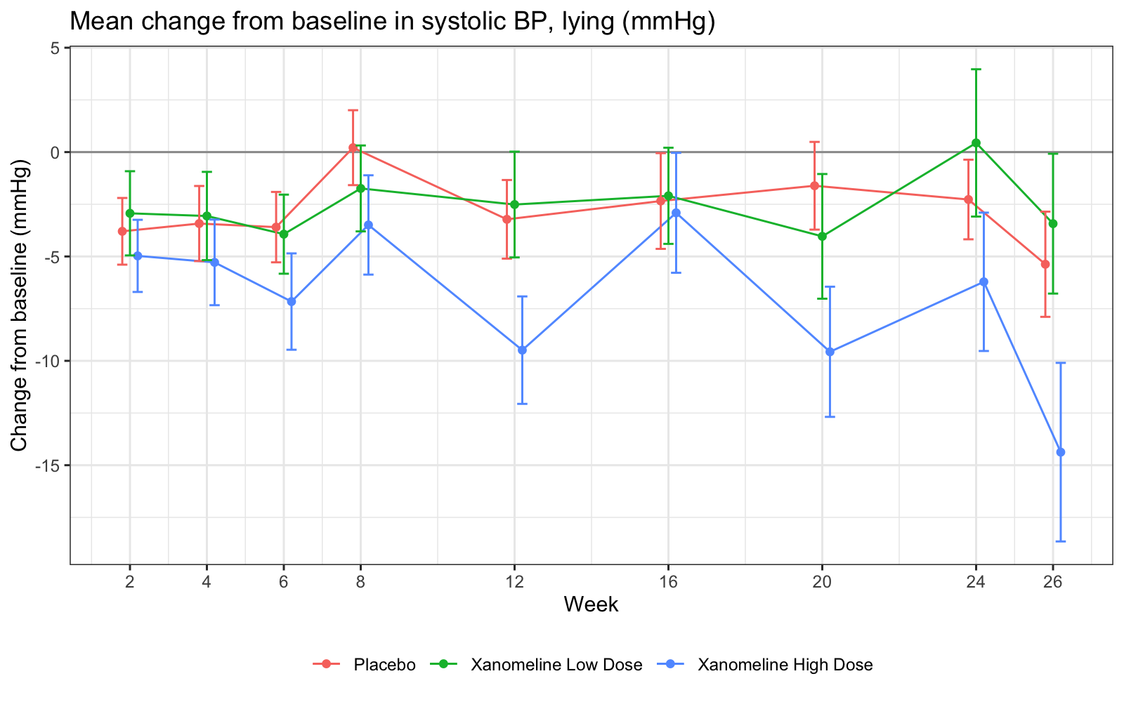
At week 24: placebo n = 59, mean change −2.27 mmHg; low dose n = 25, 0.44 mmHg; high dose n = 28, −6.21 mmHg. Only the filter() and the titles change. Blood pressure is measured in three positions, so ATPT must select one of them. The AVERAGE records have no ATPT, so this filter also removes them: there is one record per subject and visit.
Exercise 14-3
Section titled “Exercise 14-3”# Answer 14-3: the placebo subjects at risk at day 90, counted from the datalibrary(dplyr)
ttde <- readRDS("output/ttde.rds") # made by 14_4
# at risk at day 90: no event and not censored before day 90ttde |> filter(TRT == "Placebo") |> summarise(at_risk_90 = sum(AVAL >= 90))#> # A tibble: 1 x 1#> at_risk_90#> <int>#> 1 4949, as in the risk table. A subject is at risk at day 90 when the event or the censoring came on day 90 or later: AVAL >= 90. A subject with an event before day 90 left the risk set at that event; a subject censored before day 90 left it at the censoring.
Exercise 14-4
Section titled “Exercise 14-4”# Answer 14-4: a length in the specification that is too short for the datalibrary(dplyr)library(xportr)
spec <- tribble( ~dataset, ~variable, ~type, ~length, ~label, "ADSL", "USUBJID", "character", 11, "Unique Subject Identifier", "ADSL", "TRT01A", "character", 10, "Actual Treatment for Period 01")
pharmaverseadam::adsl |> filter(SAFFL == "Y") |> select(USUBJID, TRT01A) |> xportr_metadata(spec, domain = "ADSL") |> xportr_type() |> xportr_length() |> xportr_label() |> xportr_write("output/adslshrt.xpt")#> Warning message:#> Column `TRT01A` contains string values longer than user width 10. Width set to 20 to accommodate.
foreign::lookup.xport("output/adslshrt.xpt")$adsl$width#> [1] 11 20haven::read_xpt("output/adslshrt.xpt") |> distinct(TRT01A)#> # A tibble: 3 x 1#> TRT01A#> <chr>#> 1 Placebo#> 2 Xanomeline High Dose#> 3 Xanomeline Low DoseR writes a warning: Column TRT01A contains string values longer than user width 10. Width set to 20 to accommodate. The file gets the length 20, and no value is cut: read_xpt() gives the three full treatment names. The data is safe, but the file does not match the specification any more. Correct the specification, never ignore the warning: define.xml is made from the specification and would say 10.
Found an error or have a question? Write to datastep.studio@gmail.com· Every program runs in DataStep Studio for R, the R extension for VS Code and Positron.
Data: the CDISC pilot study (cdiscpilot01), from the R packagespharmaversesdtm andpharmaverseadam (Apache License 2.0).
R is a project of the R Foundation. SAS and all other SAS Institute Inc. product or service names are registered trademarks or trademarks of SAS Institute Inc. This book is not affiliated with or endorsed by SAS Institute Inc. or the R Foundation. CDISC, SDTM and ADaM are trademarks of the Clinical Data Interchange Standards Consortium.
© 2026 DataStep Labs. All rights reserved.